Quantum_fitter
This notebook shows you how to use the quantum_fitter. The purpose of quantum_fitter is to provide a uniform, easy-to-use fitting protocol, that everyone can share and extend.
Quantum_fitter builds on the lmfit package https://lmfit.github.io/lmfit-py/
To use the quantum_fitter package, you initialize an instance with your x-data, y-data, and the models you want to fit to as well as the initial guesses for parameters:
[1]:
import quantum_fitter as qf
import numpy as np
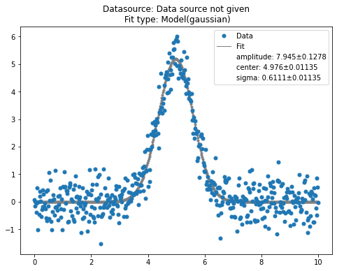
First we generate some data we can fitt
[2]:
def gaussian(x, amp, cen, wid):
    return (amp / (np.sqrt(2*np.pi) * wid)) * np.exp(-(x-cen)**2 / (2*wid**2))

# Generate random number from gaussian distribution
x = np.linspace(0, 10, 500)
y = gaussian(x, 8, 5, 0.6) + np.random.randn(500) * 0.5
Chosse model and give initial guess
Then we specify the model we want to use and the initial guess. In this example we use the ‘GaussianModel’ which is shipped with lmfit.
[3]:
params_ini = {'amplitude': 5,
              'center': 5,
              'sigma': 1}
qfit = qf.QFit(x, y,'GaussianModel', params_ini)
To fit
To perform the actual fit we call do_fit()
[4]:
qfit.do_fit()
We can inspect the result
[5]:
qfit.result
[5]:
Model
Model(gaussian)Fit Statistics
| fitting method | least_squares | |
| # function evals | 8 | |
| # data points | 500 | |
| # variables | 3 | |
| chi-square | 124.614337 | |
| reduced chi-square | 0.25073307 | |
| Akaike info crit. | -688.692216 | |
| Bayesian info crit. | -676.048391 |
Variables
| name | value | standard error | relative error | initial value | min | max | vary | expression |
|---|---|---|---|---|---|---|---|---|
| amplitude | 7.94495776 | 0.12777798 | (1.61%) | 5 | -inf | inf | True | |
| center | 4.97649272 | 0.01134850 | (0.23%) | 5 | -inf | inf | True | |
| sigma | 0.61108938 | 0.01134850 | (1.86%) | 1 | -inf | inf | True | |
| fwhm | 1.43900549 | 0.02672368 | (1.86%) | 2.35482 | -inf | inf | False | 2.3548200*sigma |
| height | 5.18676946 | 0.08341830 | (1.61%) | 1.9947115000000002 | -inf | inf | False | 0.3989423*amplitude/max(1e-15, sigma) |
Correlations (unreported correlations are < 0.100)
| amplitude | sigma | 0.5774 |
Finally we can plot the result
[6]:
plot_settings = {
    'x_label': 'Time (us)',
    'y_label': 'Voltage (mV)',
    'plot_title': 'datasource',
    'fit_color': 'C4',
    'fig_size': (8, 6)}
qfit.pretty_print()
To print the resulting plot to a pdf, use pdf_print:
[ ]:
#qfit.pdf_print('qfit.pdf')
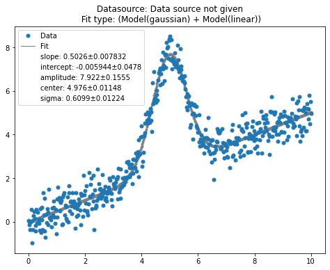
Two models on top of each other
We add a linear term to the gausian data.
[7]:
y = y + 0.5*x
[8]:
params_ini = {'intercept': 0,
              'slope': 0.5,
              'amplitude': 5,
              'center': 5,
              'sigma': 1}
qfit = qf.QFit(x, y,['GaussianModel', 'LinearModel'], params_ini)
qfit.do_fit()
qfit.pretty_print()
To get the fit parameters’ results, we can use qfit.fit_params, qfit.err_params. The method qfit.fit_values returns the y-data from the fit.
[9]:
f_p = qfit.fit_params() # return dictionary with all the fitting parameters
f_e = qfit.err_params('amplitude') # return float of amplitude's fitting stderr
y_fit = qfit.fit_values()
[27]:
qfit.params
{'amplitude': 5,
 'center': 5,
 'sigma': 1,
 'fwhm': 2.35482,
 'height': 1.9947115000000002,
 'slope': 0.5,
 'intercept': 0}
[27]:
{'amplitude': 5,
'center': 5,
'sigma': 1,
'fwhm': 2.35482,
'height': 1.9947115000000002,
'slope': 0.5,
'intercept': 0}
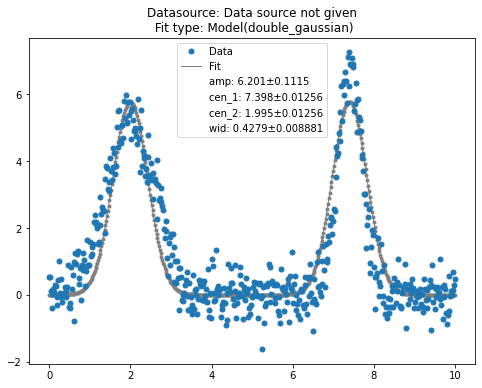
Or we can use our own modification function
[10]:
y2 = gaussian(x, 8, 2, 0.6) + gaussian(x, 5, 7.4, 0.3)+ np.random.randn(500) * 0.5
[11]:
def double_gaussian(x, amp, cen_1, cen_2, wid):
    return gaussian(x, amp, cen_1, wid) + gaussian(x, amp,cen_2, wid)
[12]:
params_ini = {'amplitude': 5,
              'center': 5,
              'sigma': 1}
qfit = qf.QFit(x, y2,double_gaussian, [5, 5, 6, 1])
qfit.do_fit()
qfit.pretty_print()
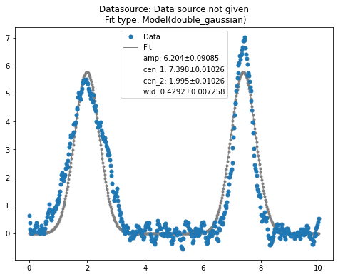
smooth the data
If need to smooth the data beforehand, use qfit.wash() to filter the spikes.
[13]:
qfit.wash(method='savgol', window_length=5, polyorder=1)
[14]:
qfit.do_fit()
qfit.pretty_print()
Appendix A: The build-in function list
Peak-like models, for more models, tap here.
To obtain the parameters in the models, use qf.params('GaussianModel') to get.